XAU / PAXG-XAUT Pairs Stationarity Analysis
Find the notebook here.This notebook will provide arbitrage indications for spot to asset-backed cryptocurrency pairs. In particular, the XAUt/USDt and PAXG/USDt pairs will be analyzed against spot gold - taking advantage of low volume pair trading. In addition, this notebook will aim to run statistical tests to identify stationarity and mean reversion.
Data Consolidation
Create a helper function to fetch the data from the pyth price oracle.
1 2 3 4 | # fetch data from the 'pyth' price oracle. import requests as req def getBarsPyth(symbol, resolution, start, end): return req.get("https://benchmarks.pyth.network/v1/shims/tradingview/history?symbol={0}&resolution={1}&from={2}&to={3}".format(symbol, resolution, start, end)).json() |
Fetch bars as objects from the helper function oracle for XAU/USD, XAUt/USD, PAXG/USD. Ensure that the start date is further than 2023-12-04 (listing date of XAUt) and is not a weekend (as XAU/USD does not trade on weekends).
1 2 3 4 5 6 7 8 9 | # fetch bars as JSON objecobject import time import datetime as dt interval = 60 # default = 60 start, end = dt.date(2024, 1, 4), dt.date.today() # default = 1/4/2024 -> today XAU = getBarsPyth("Metal.XAU%2FUSD", interval, int(time.mktime(start.timetuple())), int(time.mktime(end.timetuple()))) XAUT = getBarsPyth("Crypto.XAUT%2FUSD", interval, int(time.mktime(start.timetuple())), int(time.mktime(end.timetuple()))) PAXG = getBarsPyth("Crypto.PAXG%2FUSD", interval, int(time.mktime(start.timetuple())), int(time.mktime(end.timetuple()))) |
Data Cleaning
With the dataset from pyth, place the datasets into a dictionary to then be merged into one DataFrame, using time (in UNIX) as an index.
1 2 3 4 5 6 7 8 9 10 11 12 13 14 15 16 17 18 19 | # create timeseries as dict import pandas as pd import matplotlib.pyplot as plt xau_pair = {'t': XAU['t'], 'c_xau': XAU['c']} xaut_pair = {'t': XAUT['t'], 'c_xaut': XAUT['c']} paxg_pair = {'t': PAXG['t'], 'c_paxg': PAXG['c']} # merge data into dataframe (data) df1, df2, df3 = pd.DataFrame(xau_pair), pd.DataFrame(xaut_pair), pd.DataFrame(paxg_pair) df1.set_index('t', inplace=True) df2.set_index('t', inplace=True) df3.set_index('t', inplace=True) merged = pd.concat([df1, df2, df3], axis=1, join='outer') merged.sort_values(by='t', inplace=True) merged = merged.reset_index() merged['time'] = pd.to_datetime(merged['t'],unit='s') merged = merged.set_index('t') data = merged |
Normalize XAU, XAUt, and PAXG by taking the percent difference of the closing price of each bar.
1 2 3 4 | # adjust for price difference, normalize with pct change data['pct_c_xau'] = (data['c_xau'] / data['c_xau'].iloc[0] - 1) * 100 data['pct_c_xaut'] = (data['c_xaut'] / data['c_xaut'].iloc[0] - 1) * 100 data['pct_c_paxg'] = (data['c_paxg'] / data['c_paxg'].iloc[0] - 1) * 100 |
Calculate the spread of each datapoint with respect to XAU (w/ a XAUt-PAXG spread).
1 2 3 4 5 6 7 8 9 | # spread data['pct_c_xau_interpolated'] = data['pct_c_xau'].interpolate(method='linear') gold_i, paxg_i, xaut_i = data['pct_c_xau_interpolated'], data['pct_c_paxg'], data['pct_c_xaut'] aligned_goldGP, aligned_paxgGP = gold_i.align(paxg_i, join='outer') aligned_goldGX, aligned_xautGX = gold_i.align(xaut_i, join='outer') aligned_paxgPX, aligned_xautPX = paxg_i.align(xaut_i, join='outer') data['spread_xaupaxg'] = aligned_goldGP - aligned_paxgGP data['spread_xauxaut'] = aligned_goldGX - aligned_xautGX data['spread_xautpaxg'] = aligned_xautPX - aligned_paxgPX |
Data Analysis
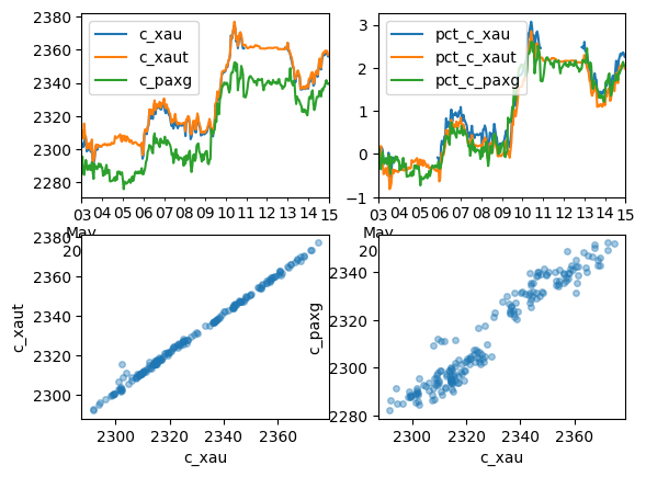
Let us plot the graph of PAXG, XAUt, and XAU - both raw and normalized; additionally plot the correlation of PAXG and XAUt with respect to XAU.
1 2 3 4 5 6 | # graph of percent changes of gold, xaut, and paxg fig, axes = plt.subplots(nrows=2, ncols=2) data.loc[:,['c_xau', 'c_xaut', 'c_paxg', 'time']].plot(x = 'time', ax=axes[0,0]) data.loc[:,['pct_c_xau', 'pct_c_xaut', 'pct_c_paxg', 'time']].plot(x = 'time', ax=axes[0,1]) data.plot(kind='scatter', x='c_xau', y='c_xaut', s=16, alpha=0.4, ax=axes[1,0]) data.plot(kind='scatter', x='c_xau', y='c_paxg', s=16, alpha=0.4, ax=axes[1,1]) |
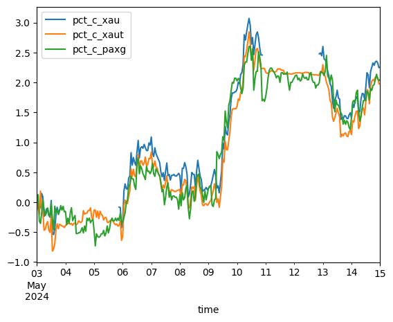
1 | data.loc[:,['pct_c_xau', 'pct_c_xaut', 'pct_c_paxg', 'time']].plot(x = 'time') |
Analytically, we can show that XAU, XAUt, and PAXG all exhibit strong correlation. Since these datasets are meant to be directly proportional to each other, any variation we exhibit in this dataset is a theoretical risk-free profit. However, before we put these claims into practice, let us perform statistical tests to prove direct proportionality, stationarity, and mean reversion.
1 | print(data.loc[:,['c_xau', 'c_xaut', 'c_paxg']].corr()) |
c_xau c_xaut c_paxg
c_xau 1.000000 0.998364 0.964174
c_xaut 0.998364 1.000000 0.971587
c_paxg 0.964174 0.971587 1.000000
As this DataFrame is from January to Mid-May, on the assumption that this data isn't mean reverting [1], the expected loss for an unleveraged portfolio would be the spread between XAUt and PAXG. However, we see a strong positive correlation. To take advantage of spread trading, let us create three datasets - the spread between XAUt, PAXG w/ respect to XAU, and a XAUt-PAXG spread.
[1] A mean reverting series is a group of data that retains 'memory' - as a series deviate from a given mean, it tends to traverse back to the mean (hence 'reverting').
1 2 3 | graph = data.copy() graph['root'] = aligned_goldGP - aligned_goldGP # this is such a bad way to initialize all zero values. graph.loc[:,['spread_xaupaxg', 'spread_xauxaut', 'spread_xautpaxg', 'root', 'time']].plot(x = 'time') |
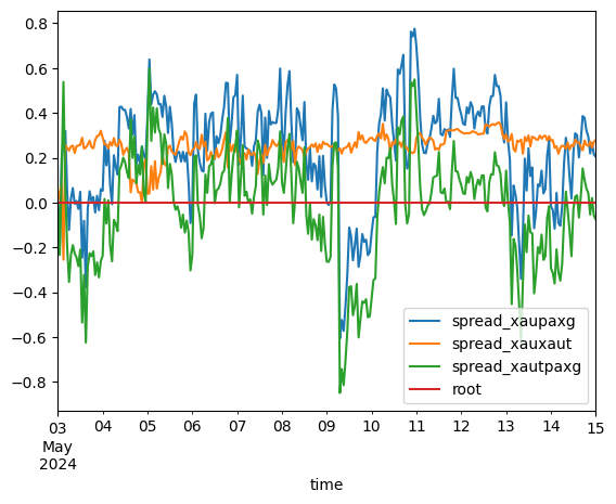
In a completely efficient market, we should expect absolutely no deviation in price - however that doesn't exist (I hate economists). To create a profit in this situation, one would short the base currency and long the trading currency (or vice versa, depending on the direction of the spread). To prove that this is truly risk-free, we must demonstrate that the PAXG, XAUT pair spreads exhibit mean reversion. A continuous mean-reverting time series can be represented by an Ornstein-Uhlenbeck stochastic differential equation:
Where \(\theta\) is the rate of reversion to the mean, \(\mu\) is the mean value of the process, \(\sigma\) is the variance of the process, and \(W_t\) is a Wiener Process or a Brownian Motion. In a discrete setting, the equation states that the change of the price series in the next time period is proportional to the difference between the mean price and the current price, with the addition of Gaussian noise. This motivates the Augmented Dickey-Fuller Test, which we will describe below.
Augmented Dickey-Fuller Test
A unit root is a stochastic trend in a given series. The point of an Augmented Dickey-Fuller Test is to determine whether or not a unit root exists; if it does not exist, the series is not trending. As a result, a higher score in the Dickey-Fuller test indicates that there's a more prominent trend, and vice versa.
1 2 3 4 5 6 7 8 | import statsmodels.tsa.stattools as ts adf_xauxaut = ts.adfuller(data['spread_xauxaut'], 1) # perform adf on xau-xaut adf_xaupaxg = ts.adfuller(data['spread_xaupaxg'], 1) # perform adf on xau-paxg adf_xautpaxg = ts.adfuller(data['spread_xautpaxg'], 1) # perform adf on xaut-paxg print("adfuller for XAU-XAUT: {0}".format(adf_xauxaut)) print("adfuller for XAU-PAXG: {0}".format(adf_xaupaxg)) print("adfuller for XAUT-PAXG: {0}".format(adf_xautpaxg)) print(type(adf_xaupaxg)) |
adfuller for XAU-PAXG: (-5.735268089050287, 6.460192127149706e-07, 0, 288, {'1%': -3.453261605529366, '5%': -2.87162848654246, '10%': -2.5721455328896603}, -304.917811118788)
adfuller for XAUT-PAXG: (-5.729545258695016, 6.649327955430402e-07, 0, 288, {'1%': -3.453261605529366, '5%': -2.87162848654246, '10%': -2.5721455328896603}, -277.07578574419176)
<class 'tuple'>
The ts.adfuller() API calls for returning a tuple with the following attributes:
| Value | Description |
|---|---|
adf : float |
Test statistic |
pvalue: float |
MacKinnon’s approximate p-value based on MacKinnon (1994, 2010) |
usedlag: int |
Number of lags used |
nobs: int |
Number of observations used for the ADF regression and calculation of the critical values |
critical values: dict |
Critical values for the test statistic at the 1%, 5%, and 10% levels. Based on MacKinnon (2010) |
icbest: float |
The maximized information criterion if autolag is not None. |
As noted in the output [ref], all of our series have a \(p\)-value lower than \(0.01\), which is promising (we can now reject the null hypothesis of \(\gamma = 1\)). Let us reverify our observation by finding the Hurst Exponent.
Hurst Exponent
The Hurst exponent (HE) aims to provide us a scalar value that helps us identify the 'memory' of a series (i.e. mean reversion). A series with \(HE > 0.5\) is said to be trending, \(HE = 0.5\) is said to be GBM (random walk), and \(HE < 0.5\) is categorized as mean reverting.
1 2 3 4 5 6 7 8 9 10 11 12 13 14 | # create hurst exponent function import numpy as np from numpy import cumsum, log, polyfit, sqrt, std, subtract # input is numpy array def hurst(ts): lags = range(2, 100) # create the range of lagging values tau = [sqrt(std(subtract(ts[lag:], ts[:-lag]))) for lag in lags] # variance m = polyfit(log(lags), log(tau), 1) # polynomial fit return m[0] * 2 # return exponent print("hurst(XAU-XAUT): {0}".format(hurst(data['spread_xauxaut'].values))) print("hurst(XAU-PAXG): {0}".format(hurst(data['spread_xaupaxg'].values))) print("hurst(XAUT-PAXG): {0}".format(hurst(data['spread_xautpaxg'].values))) |
hurst(XAU-PAXG): 0.1254107697763245
hurst(XAUT-PAXG): 0.11409796976657859
Nice.